Merger Tree Mass Distributions

Class providing the sampling rate (trees per decade of halo mass) as a function of halo mass and time, used when drawing a set of merger tree root masses. The sampling distribution determines how many trees are built at each mass, and implementations typically follow the halo mass function to ensure representative sampling. The sampling rate is used together with assigned statistical weights so that volume-averaged quantities (e.g.galaxy stellar mass functions) can be correctly computed.

Default implementation: mergerTreeBuildMassDistributionHaloMassFunction

Methods

sample → double precision

Returns the sampling rate for merger trees of the given mass, per decade of halo mass.

• double precision, intent(in ) :: mass,time,massMinimum,massMaximum

mergerTreeBuildMassDistributionGaussian

A merger tree halo mass function sampling class in which the sampling rate is given by a Gaussian distribution in halo mass.

Parameters

• [mean] — The mean mass of halo to simulate when using a Gaussian sampling of the halo mass function.

• [rootVariance] — The dispersion in mass of halo to simulate when using a Gaussian sampling of the halo mass function.

mergerTreeBuildMassDistributionHaloMassFunction

A merger tree build mass distribution class in which the sampling density function equal to the halo mass function,

\[\gamma(M) = \hbox{minmax}(\phi_\mathrm{min},\phi_\mathrm{max},\mathrm{d} n(M)/\mathrm{d}\log M [1 + p_1 \log_{10}(M/10^{13}\mathrm{M}_\odot) + p_2 \log_{10}^2(M/10^{13}\mathrm{M}_\odot)),\]

where \(\phi_\mathrm{min}=\)[abundanceMinimum], \(\phi_\mathrm{max}=\)[abundanceMaximum], \(p_1=\)[modifier1], \(p_2=\)[modifier2], and

\[\begin{split}\hbox{minmax}(a,b,x) = \left\{\begin{array}{ll}a & \hbox{ if } x < a \\ x & \hbox{ if } a \leq x \leq b\\ b & \hbox{ if } x > b,\end{array}\right.\end{split}\]

resulting in a sample of halos representative of a volume of space.

(Default implementation)

Methods

• descriptorSpecial — Handle adding special parameters to the descriptor.

Parameters

• [abundanceMinimum] (default -1.0d0) — The abundance (in units of Mpc\(^{-3}\)) below which to truncate the halo mass function when sampling halo masses for tree construction. A negative value indicates no truncation.

• [abundanceMaximum] (default -1.0d0) — The abundance (in units of Mpc\(^{-3}\)) above which to truncate the halo mass function when sampling halo masses for tree construction. A negative value indicates no truncation.

• [modifier1] (default 0.0d0) — Coefficient of the polynomial modifier applied to the halo mass function when sampling halo masses for tree construction.

• [modifier2] (default 0.0d0) — Coefficient of the polynomial modifier applied to the halo mass function when sampling halo masses for tree construction.

• [baseParametersFileName] — The path to the XML parameter file that provides the base configuration for each model evaluation, to which parameter changes from the posterior sampler are then applied.

• [pathSamples] (default var_str('none')) — The path into which the sampled mass functions should be written. If none, then samples are not written.

• [appendSamples] (default .false.) — If true, samples will be appended to the file. Otherwise, the file is overwritten.

• [fileNames] — The names of the files containing the halo mass functions.

• [redshifts] — The redshifts at which to evaluate the halo mass functions.

• [massRangeMinimum] — The minimum halo mass to include in the likelihood evaluation.

• [massRangeMaximum] (default huge(0.0d0)) — The maximum halo mass to include in the likelihood evaluation.

• [binCountMinimum] — The minimum number of halos per bin required to permit bin to be included in likelihood evaluation.

• [likelihoodPoisson] (default .false.) — If true, likelihood is computed assuming a Poisson distribution for the number of halos in each bin (with no covariance between bins). Otherwise a multivariate normal is assumed when computing likelihood.

• [varianceFractionalModelDiscrepancy] (default 0.0d0) — The fractional variance due to model discrepancy.

• [allowEmptyMassFunction] (default .false.) — If true, empty mass functions (i.e. those with no useable bins) are allowed, and return \(\log \mathcal{L}=0\).

• [report] (default .false.) — If true, give detailed reporting on likelihood calculations.

• [includeCorrelations] (default .false.) — If true, account for correlations between halo mass functions measured at different redshifts.

• [binAverage] (default .true.) — If true, the mass function is averaged over each bin.

• [changeParametersFileNames] — The names of files containing parameter changes to be applied.

• [haloMassMinimum] (default 1.0d10) — The minimum mass at which to tabulate halo mass functions.

• [haloMassMaximum] (default 1.0d15) — The maximum mass at which to tabulate halo mass functions.

• [pointsPerDecade] (default 10.0d0) — The number of points per decade of halo mass at which to tabulate halo mass functions.

• [outputGroup] (default var_str('.')) — The HDF5 output group within which to write mass function data.

• [includeUnevolvedSubhaloMassFunction] (default .false.) — If true then also compute and output the unevolved subhalo mass function.

• [includeMassAccretionRate] (default .true.) — If true then also compute and output the mass accretion rate of the halos.

• [massesRelativeToHalfModeMass] (default .false.) — If true then masses are interpreted (and output) relative to the half-mode mass. (If the half-mode mass is undefined an error will occur.) If false, masses are absolute.

• [errorsAreFatal] (default .true.) — If true then errors in evaluating the halo mass function are considered to be fatal.

• [labels] — Labels for virial density contrast mass definitions.

• [fractionModeMasses] — List of suppression fractions at which to compute the fractional mode mass.

mergerTreeBuildMassDistributionPowerLaw

A merger tree build mass distribution class in which the sampling rate is given by a power-law in halo mass. Specifically:

\[\gamma(M) = \log_{10}(M/M_\mathrm{minimum})^{-\alpha/(1+\alpha)},\]

The resulting distribution of halo masses is such that the mass of the \(i^\mathrm{th}\) halo is

\[M_\mathrm{halo,i} = \exp\left[ \ln(M_\mathrm{halo,min}) + \ln\left({M_\mathrm{halo,max}/M_\mathrm{halo,min}}\right) x_i^{1+\alpha} \right].\]

Here, \(x_i\) is a number between 0 and 1 and \(\alpha=\)[exponent] is an input parameter that controls the relative number of low and high mass tree produced.

Parameters

• [exponent] (default 1.73d0) — Exponent of the differential luminosity function.

• [rateHydrogenIonizingPhotonsMinimum] (default 1.0d48) — The minimum ionizing photon production rate (\(Q_\mathrm{H,min}\), in photons/s) below which the power-law HII region luminosity function is truncated to zero.

• [rateHydrogenIonizingPhotonsMaximum] (default huge(0.0d0)) — The maximum ionizing photon production rate (\(Q_\mathrm{H,max}\), in photons/s) above which the power-law HII region luminosity function is truncated to zero.

• [exponent] (default 1.0d0) — Halo masses will be (pseudo-)uniformly distributed in \([\log(M)]^{1/(1+\alpha)}\) where \(\alpha=\)exponent.

• [wavelengthMinimum] — The minimum wavelength (in units of AA) for the power-law spectrum.

• [wavelengthMaximum] — The maximum wavelength (in units of AA) for the power-law spectrum.

• [exponent] — The exponent of the power-law spectrum.

• [normalization] — The normalization (in units of \(L_\odot / \AA\)) of the power-law spectrum.

• [normalization] — Parameter \(\sigma_{12}\) appearing in model for random errors in the halo mass function.

• [fractionalErrorHighMass] — Parameter \(\sigma_\infty\) appearing in model for random errors in the halo mass function.

• [exponent] — Parameter \(\gamma\) appearing in model for random errors in the halo mass function. Specifically, the fractional error is given by \(\sigma(M) = \left[ \sigma^2_{12} \left({M_\mathrm{halo} \over 10^{12}\mathrm{M}_\odot}\right)^{2\gamma} + \sigma^2_\infty \right]^{1/2}\), where \(\sigma_{12}=\)[normalization] and \(\gamma=\)[exponent].

• [correlationModelTrivial] (default .true.) — If true, the correlation between mass errors of pairs of halos is unity for halos with identical mass and time, and zero otherwise. If false, a power-law correlation model in mass ratio and expansion factor ratio is used instead.

• [correlationNormalization] (default 0.0d0) — Variable \(C_0\) in the model for the correlation between halo mass errors: \(C_{12} = C_0 [M_2/M_1]^\alpha [(1+z_2)/(1+z_1)]^\beta\).

• [correlationMassExponent] (default 0.0d0) — Variable \(\alpha\) in the model for the correlation between halo mass errors: \(C_{12} = C_0 [M_2/M_1]^\alpha [(1+z_2)/(1+z_1)]^\beta\).

• [correlationRedshiftExponent] (default 0.0d0) — Variable \(\beta\) in the model for the correlation between halo mass errors: \(C_{12} = C_0 [M_2/M_1]^\alpha [(1+z_2)/(1+z_1)]^\beta\).

• [radiusLow] (default +0.0154d0) — The low-mass limit of the characteristic scale radius \(r_0\) (in Mpc) in the power-law scale radius model, giving the scale radius normalization for low-mass halos as a function of peak height and expansion factor.

• [radiusHigh] (default +0.0962d0) — The high-mass limit of the characteristic scale radius \(r_1\) (in Mpc) in the power-law scale radius model, giving the scale radius normalization for high-mass halos.

• [radiusTransition] (default +1.2137d0) — The peak height \(\nu\) at which the characteristic scale radius transitions between its low-mass and high-mass limiting values in the power-law scale radius model.

• [radiusWidth] (default +0.5482d0) — The parameter \(\Delta r\) in the power-law scale radius model.

• [massLow] (default +0.3895d0) — The parameter \(\alpha_0\) in the power-law scale radius model.

• [massHigh] (default +0.2984d0) — The parameter \(\alpha_1\) in the power-law scale radius model.

• [massTransition] (default -0.2583d0) — The parameter \(\alpha_\nu\) in the power-law scale radius model.

• [massWidth] (default +16.6050d0) — The parameter \(\Delta \alpha\) in the power-law scale radius model.

• [expansionFactorLow] (default -0.6977d0) — The parameter \(\beta_0\) in the power-law scale radius model.

• [expansionFactorHigh] (default +0.7972d0) — The parameter \(\beta_1\) in the power-law scale radius model.

• [expansionFactorTransition] (default +0.5395d0) — The parameter \(\beta_\nu\) in the power-law scale radius model.

• [expansionFactorWidth] (default +0.4282d0) — The parameter \(\Delta \beta\) in the power-law scale radius model.

• [scatter] (default +0.1513d0) — The scatter (in dex) in the scale radius at fixed halo mass and redshift in the power-law scale radius model, representing the intrinsic halo-to-halo variation in concentration.

• [index] (default 0.9649d0) — The index of the power-law primordial power spectrum.

• [running] (default 0.0d0) — The running, \(\d n_\mathrm{s} / \d \ln k\), of the power spectrum index.

• [runningRunning] (default 0.0d0) — The running-of-the-running, \(\d^2 n_\mathrm{s} / \d \ln k^2\), of the power spectrum index.

• [wavenumberReference] (default 1.0d0) — When a running power spectrum index is used, this is the wavenumber, \(k_\mathrm{ref}\), at which the index is equal to [index].

• [runningSmallScalesOnly] (default .false.) — If true then the index runs only for \(k > k_\mathrm{ref}\), for smaller \(k\) the index is constant.

mergerTreeBuildMassDistributionStllrMssFnctn

A merger tree build mass distribution class designed to minimize variance in the model stellar mass function.

Suppose we want to fit parameters of the Galacticus model to some dataset. The basic approach is to generate large numbers of model realizations for different parameter values and see which ones best match the data. Galacticus models involve simulating individual merger trees and then adding together their galaxies to produce some overall function. The question we want to answer is, given some finite amount of computing time, what is the optimal distribution of halo masses to run when comparing to a given dataset. For example, is it better to run a volume limited sample (as one would get from an N-body simulation) or is it better to use, say, equal numbers of halos per logarithmic interval of halo mass? The following section describes how to solve this optimization problem in the specific case of fitting to the stellar mass function.

First, some definitions:

\(n(M) \d \ln M\)

is the dark matter halo mass function, i.e. the number of halos in the range \(M\) to \(M+M\d\ln M\) per unit volume;

\(\gamma(M) \d \ln M\)

is the number of trees that we will simulate in the range \(M\) to \(M+M\d \ln M\);

\(\alpha(M_\star)\)

is the error on the observed stellar mass function at mass \(M_\star\);

\(P(N|M_\star,M;\delta \ln M_\star)\)

is the conditional stellar mass distribution function of galaxies of stellar mass \(M_\star\) in a bin of width \(\delta \ln M_\star\) per halo of mass \(M\);

\(t(M)\)

is the CPU time it takes to simulate a tree of mass \(M\).

To clarify, \(P(N|M_\star,M;\delta \ln M_\star;\delta \ln M_\star)\) is the probabilityfootnoteTo put it another way, \(P(N|M_\star,M;\delta \ln M_\star)\) is closely related to the commonly used Halo Occupation Distribution. to find \(N\) galaxies of mass between \(M_\star\) in a bin of width \(\delta \ln M_\star\) in a halo of mass \(M\). The usual conditional stellar mass function is simply the first moment of this distribution:

(17)\[\phi(M_\star;M) \delta \ln M_\star = \sum_{N=0}^\infty N P(N|M_\star,M;\delta \ln M_\star)\]

The model estimate of the stellar mass function \(\Phi(M_\star)\) (defined per unit \(\ln M_\star\)) is

\[\Phi(M_\star) = \int_0^\infty \phi(M_\star;M) {n(M) \over \gamma(M)} \gamma(M) \d \ln M,\]

where the \(n(M)/\gamma(M)\) term is the weight assigned to each tree realization—and therefore the weight assigned to each model galaxy when summing over a model realization to construct the stellar mass function.

When computing a model likelihood, we must employ some statistic which defines how likely the model is given the data. Typically, for stellar mass functions we have an estimate of the variance in the data, \(\alpha^2(M_\star)\), as a function of stellar mass (full covariance matrices are typically not provided but, ideally would be, and can be easily incorporated into this method). In that case, we can define a likelihood

\[\ln \mathcal{L} = - {1 \over 2} \sum_i {[\phi_{\mathrm{obs},i} - \phi_i]^2 \over \alpha_i^2 + \sigma_i^2}\]

where the sum is taken over all data points, \(i\), and \(\sigma_i^2\) is the variance in the model estimate and is given by

\[\sigma^2(M_\star) = \langle [\phi(M_\star) - \bar{\phi}(M_\star)]^2 \rangle,\]

where \(\phi(M_\star)\) is the realization from a single model and \(\bar{\phi}(M_\star)\) is the model expectation from an infinite number of merger tree realizations and the average is taken over all possible model realizations. Since the contributions from each merger tree are independent,

\[\sigma^2(M_\star) = \sum_i \zeta_i^2(M_\star;M)\]

where \(\zeta_i^2(M_\star;M)\) is the variance in the contribution to the stellar mass function from tree \(i\). This in turn is given by

\[\zeta^2(M_\star;M) = \psi^2(M_\star;M) \left[{n(M) \over \gamma(M)}\right]^2,\]

where \(\psi^2(M_\star;M)\) is the variance in the conditional stellar mass function. In the continuum limit this becomes

\[\sigma^2(M_\star) = \int_0^\infty \psi^2(M_\star;M) \left[{n(M) \over \gamma(M)}\right]^2 \gamma(M) \d \ln M.\]

Model variance artificially increases the likelihood of a given model. We would therefore like to minimize the increase in the likelihood due to the model variance:

\[\Delta 2 \ln \mathcal{L} = \sum_i {[\phi_{\mathrm{obs},i} - \phi_i]^2 \over \alpha_i^2} - {[\phi_{\mathrm{obs},i} - \phi_i]^2 \over \alpha_i^2 + \sigma_i^2}\]

Of course, we don’t know the model prediction, \(\phi_i\), in advancefootnoteBelow, we will adopt a simple empirical model for \(\phi(M_\star)\). However, it should not be used here since we will in actuality be computing the likelihood from the model itself.. However, if we assume that a model exists which is a good fit to the data then we would expect that \([\phi_{\mathrm{obs},i} - \phi_i]^2 \approx \alpha_i^2\) on average. In that case, the increase in likelihood due to the model is minimized by minimizing the functionfootnoteThis can be seen intuitively: we are simply requiring that the variance in the model prediction is small compared the the variance in the data.

\[F[\gamma(M)] = \sum_i {\alpha_i^2 \over \alpha_i^2 + \sigma_i^2}.\]

If the bins all have the same \(\delta \ln M_\star\) we can turn the sum into an integral

\[F[\gamma(M)] = \int_0^\infty {\alpha(M_\star)^2 \over \alpha(M_\star)^2 + \sigma(M_\star)^2} \d \ln M_\star.\]

Obviously, the answer is to make \(\gamma(M)=\infty\), in which case \(F[\gamma(M)]=0\). However, we have finite computing resources. The total time to run our calculation is

\[\tau = \int_0^\infty t(M) \gamma(M) \d \ln M.\]

We therefore want to minimize \(F[\gamma(M)]\) while keeping \(\tau\) equal to some finite value. We can do this using a Lagrange multiplier and minimizing the function

\[F[\gamma(M)] = \int_0^\infty {\alpha(M_\star)^2 \over \alpha(M_\star)^2 + \sigma(M_\star)^2} \d \ln M_\star + \int_0^\infty \lambda \gamma(M) t(M) \d \ln M.\]

Finding the functional derivative and setting it equal to zero gives:

\[\gamma(M) = \sqrt{{\xi(M) \over \lambda t(M)}},\]

in the limit wherefootnoteThis is the limit in which we would like our results to be. \(\sigma(M_\star) \ll \alpha(M_\star)\), and where

\[\xi(M) = n^2(M) \int_{-\infty}^\infty {\psi^2(M_\star;M) \over \alpha^2(M_\star)} \d \ln M_\star.\]

The values of \(\lambda\) and \(\delta \ln M_\star\), and the normalization of \(t(M)\) are unimportant here since we merely want to find the optimal shape of the \(\gamma(M)\) function—we can then scale it up or down to use the available time.

Figure 4 shows the function \(\gamma(M)\) obtained by adopting a model conditional stellar mass function which is a sum of central and satellite terms. Specifically, we use the model of Leauthaud et al. (2012) which is constrained to match observations from the COSMOS survey. In their modelfootnoteThis integral form of the conditional stellar mass function is convenient here since it allows for easy calculation of the number of galaxies expected in the finite-width bins of the observed stellar mass function.:

\[\langle N_\mathrm{c}(M_\star|M)\rangle \equiv \int_{M_\star}^\infty \phi_\mathrm{c}(M_\star^\prime) \d \ln M_\star^\prime = {1 \over 2} \left[ 1 - \hbox{erf}\left( {\log_{10}M_\star - \log_{10} f_\mathrm{SHMR}(M) \over \sqrt{2}\sigma_{\log M_\star}} \right) \right].\]

Here, the function \(f_\mathrm{SHMR}(M)\) is the solution of

\[\log_{10}M = \log_{10}M_1 + \beta \log_{10}\left({M_\star \over M_{\star,0}}\right) + {(M_\star/M_{\star,0})^\delta \over 1 + (M_\star/M_{\star,0})^{-\gamma}} - {1/2}.\]

For satellites,

\[\langle N_\mathrm{s}(M_\star|M)\rangle \equiv \int_{M_\star}^\infty \phi_\mathrm{s}(M_\star^\prime) \d \ln M_\star^\prime = \langle N_\mathrm{c}(M_\star|M)\rangle \left({f^{-1}_\mathrm{SHMR}(M_\star) \over M_\mathrm{sat}}\right)^{\alpha_\mathrm{sat}} \exp\left(- {M_\mathrm{cut} \over f^{-1}_\mathrm{SHMR}(M_\star)} \right),\]

where

\[{M_\mathrm{sat} \over 10^{12} \mathrm{M}_\odot} = B_\mathrm{sat} \left({f^{-1}_\mathrm{SHMR}(M_\star) \over 10^{12} \mathrm{M}_\odot}\right)^{\beta_\mathrm{sat}},\]

and

\[{M_\mathrm{cut} \over 10^{12} \mathrm{M}_\odot} = B_\mathrm{cut} \left({f^{-1}_\mathrm{SHMR}(M_\star) \over 10^{12} \mathrm{M}_\odot}\right)^{\beta_\mathrm{cut}}.\]

We use the best fit parameters from the SIG_MOD1 method of Leauthaud et al. (2012) for their \(z_1\) sample, but apply a shift of \(-0.2\) dex in masses to bring the fit into line with the \(z=0.07\) mass function of Li and White (2009). The resulting parameter values are shown in Table 4.

Table 4 Parameters of the conditional stellar mass function fit.

Parameter	Value
\(\alpha_\mathrm{sat}\)	1.0
\(\log_{10} M_1\)	12.120
\(\log_{10} M_{\star,0}\)	10.516
\(\beta\)	0.430
\(\delta\)	0.5666
\(\gamma\)	1.53
\(\sigma_{\log M_\star}\)	0.206
\(B_\mathrm{cut}\)	0.744
\(B_\mathrm{sat}\)	8.00
\(\beta_\mathrm{cut}\)	\(-\)0.13
\(\beta_\mathrm{sat}\)	0.859

We assume that \(P_\mathrm{s}(N|M_\star,M;\delta \ln M_\star)\) is a Poisson distribution while \(P_\mathrm{c}(N|M_\star,M;\delta \ln M_\star)\) has a Bernoulli distribution, with each distribution’s free parameter fixed by the constraint of eqn. ((17)), and the assumed forms for \(\phi_\mathrm{c}\) and \(\phi_\mathrm{s}\).

The errors in the Li and White (2009) observed stellar mass function are well fit by (see Fig. 3):

(18)\[\alpha(M_\star) = 10^{-3} \left({M_\star\over 4.5\times 10^{10}\mathrm{M}_\odot}\right)^{-0.3} \exp\left(-{M_\star\over 4.5\times 10^{10}\mathrm{M}_\odot}\right) + 10^{-7},\]

and the tree processing time in Galacticus can be described by:

\[\log_{10} t(M) = \sum_{i=0}^2 C_i [ \log_{10} M ]^i\]

with \(C_0=-0.73\), \(C_1=-0.20\) and \(C_2=0.035\).

The resulting optimal sampling density curve is shown in Fig. 4 and is compared to weighting by the halo mass function (i.e. the result of sampling halos at random from a representative volume). Optimal sampling gives less weight to low mass halos (since a sufficient accuracy can be obtained without the need to run many tens of thousands of such halos) and to high mass halos which are computationally expensive.

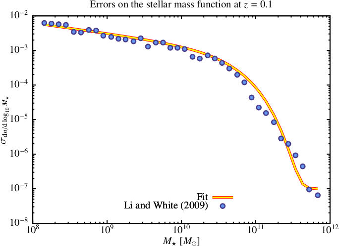
Fig. 3 Errors on the Li and White (2009) stellar mass function (points) and the fitting function (line) given by eqn. ((18)).

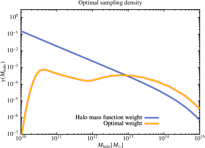
Fig. 4 Optimal weighting (yellow line) compared with weighting by the dark matter halo mass function (i.e. sampling halos at random from a representative volume; blue line). Sampling densities have been normalized to unit compute time.

Methods

• finalizeAnalysis — Finalize analysis.

Parameters

• [normalization] — The value \(\phi_0\) in a Schechter function, \(\sigma(M) = \phi_0 (M/M_\star)^\alpha \exp(-[M/M_\star]^\beta)\), describing the errors on the stellar mass function to be assumed when computing the optimal sampling density function for tree masses.

• [alpha] — The value \(\alpha\) in a Schechter function describing the errors on the stellar mass function to be assumed when computing the optimal sampling density function for tree masses.

• [beta] — The value \(\beta\) in a Schechter function describing the errors on the stellar mass function to be assumed when computing the optimal sampling density function for tree masses.

• [massCharacteristic] — The value \(M_\star\) in a Schechter function describing the errors on the stellar mass function to be assumed when computing the optimal sampling density function for tree masses.

• [constant] — The constant error contribution to the stellar mass function to be assumed when computing the optimal sampling density function for tree masses.

• [binWidthLogarithmic] — The logarithmic width of bins in the stellar mass function to be assumed when computing the optimal sampling density function for tree masses.

• [massMinimum] — The minimum stellar mass to consider when computing the optimal sampling density function for tree masses.

• [massMaximum] — The minimum stellar mass to consider when computing the optimal sampling density function for tree masses.

• [negativeBinomialScatterFractional] (default 0.18d0) — The fractional scatter (relative to the Poisson scatter) in the negative binomial distribution used in likelihood calculations.

• [randomErrorMinimum] (default 0.1d0) — The minimum random error for stellar masses.

• [randomErrorMaximum] (default 0.1d0) — The minimum random error for stellar masses.

• [randomErrorPolynomialCoefficient] (default [0.07d0]) — The coefficients of the random error polynomial for stellar masses.

• [systematicErrorPolynomialCoefficient] (default [0.0d0]) — The coefficients of the systematic error polynomial for stellar masses.

• [covarianceBinomialBinsPerDecade] (default 10) — The number of bins per decade of halo mass to use when constructing Local Group stellar mass function covariance matrices for main branch galaxies.

• [covarianceBinomialMassHaloMinimum] (default 1.0d8) — The minimum halo mass to consider when constructing Local Group stellar mass function covariance matrices for main branch galaxies.

• [covarianceBinomialMassHaloMaximum] (default 1.0d16) — The maximum halo mass to consider when constructing Local Group stellar mass function covariance matrices for main branch galaxies.

• [positionType] (default var_str('orbital')) — The type of position to use in survey geometry filters.

• [logLikelihoodZero] (default logImprobable) — The log-likelihood to assign to bins where the model expectation is zero.