Survey Geometry

Class providing galaxy survey geometries—the selection function of an observed galaxy sample, including the survey solid angle, the minimum and maximum detection distances as a function of galaxy mass, luminosity, or star formation rate, and the 3-D window functions needed for clustering analyses. These quantities are used in the on-the-fly output analysis classes to compute galaxy stellar mass functions, luminosity functions, and two-point correlation functions by applying the appropriate \(V_\mathrm{max}\) weighting and survey volume corrections.

Default implementation: surveyGeometryLiWhite2009SDSS

Methods

fieldCount → integer

Returns the number of distinct fields included in the survey.

distanceMinimum → double precision

Returns the minimum distance (in Mpc) at which a galaxy of the specified mass (in \(\mathrm{M}_\odot\)) would be included in the survey.

• double precision, intent(in ), optional :: mass , magnitudeAbsolute, luminosity, starFormationRate

• integer , intent(in ), optional :: field

distanceMaximum → double precision

Returns the maximum distance (in Mpc) at which a galaxy of the specified mass (in \(\mathrm{M}_\odot\)) could be detected.

• double precision, intent(in ), optional :: mass , magnitudeAbsolute, luminosity, starFormationRate

• integer , intent(in ), optional :: field

solidAngle → double precision

Return the solid angle (in steradians) of the survey.

• integer, intent(in ), optional :: field

volumeMaximum → double precision

Returns the maximum volume (in Mpc\(^3\)) at which a galaxy of the specified mass (in \(\mathrm{M}_\odot\)) could be detected.

• double precision, intent(in ) :: mass

• integer , intent(in ), optional :: field

windowFunctionAvailable → logical

Returns true if survey 3-D window functions are available.

angularPowerAvailable → logical

Returns true if angular power spectrum of survey window function is available.

windowFunctions → void

Returns the window functions on a grid of the specified size (gridCount cells in each dimension) for galaxies of the specified mass1 and mass2 (in \(\mathrm{M}_\odot\)). The boxLength should be set to an appropriate value to fully enclose (with sufficient buffering to allow for Fourier transformation) the two window functions.

• double precision , intent(in ) :: mass1 , mass2

• integer , intent(in ) :: gridCount

• double precision , intent( out) :: boxLength

• complex (c_double_complex), intent( out), dimension(gridCount,gridCount,gridCount) :: windowFunction1, windowFunction2

angularPower → double precision

Return \(C^{ij}_\ell\), where \((2\ell+1) C^{ij}_\ell = \sum_{m=-\ell}^{+\ell} \Psi^i_{\ell m} \Psi^{j*}_{\ell m}\), and \(\Psi^i_{\ell m}\) are the coefficients of the spherical harmonic expansion of the \(i^\mathrm{th}\) field.

• integer, intent(in ) :: i,j,l

angularPowerMaximumDegree → integer

Return the maximum degree, \(\ell_\mathrm{max}\), for which the angular power is available.

pointIncluded → logical

Return true if the given Cartesian point lies within the survey bounds for the given mass limit.

• double precision, intent(in ), dimension(3) :: point

• double precision, intent(in ) :: mass

surveyGeometryBaldry2012GAMA

A survey geometry class that describes the survey geometry of Baldry et al. (2012).

For the angular mask we use the specifications of the G09, G12, and G15 fields given by Driver et al. (2011) to construct mangle polygon files.

To determine the depth as a function of stellar mass, we make use of the publicly available tabulated mass function, \(\phi\), and number of galaxies per bin, \(N\). The effective volume of each bin is found as \(V_i = N_i/\phi_i\Delta\log_{10}M_\star\), where \(\Delta\log_{10}M_\star\) is the width of the bin. The GAMA survey consists of three fields, each of the same solid angle, but with differing depths. We assume that the relative depths in terms of stellar mass scale with the depth in terms of flux. Given this assumption, these volumes are converted to maximum distances in each field using the solid angle quoted above. The resulting mass vs. distance relation in each field is fit with a \(1^\mathrm{st}\)-order polynomial in log-log space over the range where the maximum volume is limited by the survey depth and not by the imposed \(z=0.06\) upper limit to redshift. Figure 7 shows the resulting relation between stellar mass and the maximum distance at which such a galaxy would be included in the sample. Points indicate results from GAMA, while the line shows a polynomial fit:

(20)\[\begin{split}\log_{10} \left[ {D_\mathrm{max}(M_\star) \over \hbox{Mpc}}\right] = \left\{ \begin{array}{ll} -0.521 + 0.319m & \hbox{fields G09/G15} \\ -0.361 + 0.319m & \hbox{field G12} \end{array} \right.\end{split}\]

where \(m= \log_{10}(M_\star/\mathrm{M}_\odot)\). We use this polynomial fit to determine the depth of the sample as a function of stellar mass.

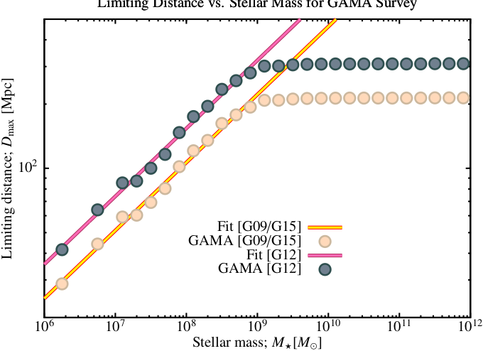
Fig. 7 The maximum distance at which a galaxy of given stellar mass can be detected in the sample of Baldry et al. (2012). Points show the results obtained from data provided by Baldry, while the lines shows a polynomial fit to these results (given in eqn. (20)). Note that above \(10^9\mathrm{M}_\odot\) the distance is limited by the imposed upper limit of \(z=0.06\) in the GAMA sample—the polynomial fit does not consider these points.

surveyGeometryBernardi2013SDSS

A survey geometry class that describes the survey geometry of Bernardi et al. (2013).

For the angular mask, we make use of the mangle polygon file provided by the mangle projectfootnoteSpecifically, https://zenodo.org/records/10998446/files/sdss_dr72safe0_res6d.pol.gz. The solid angle of this mask, computed using the mangle harmonize command is 2.232262776405 sr.

To determine the depth as a function of stellar mass, we make use of results provided by M. Bernardi (private communication), giving the mean maximum volume, \(V_\mathrm{max}\), as a function of stellar mass for galaxies in this sample. These maximum volumes are converted to maximum distances using the solid angle quoted above. The results mass vs. distance relation is fit with a \(5^\mathrm{th}\)-order polynomial. Figure 8 shows the resulting relation between stellar mass and the maximum distance at which such a galaxy would be included in the sample. Points indicate results from Bernardi, while the line shows a polynomial fit:

(21)\[\log_{10} \left[ {D_\mathrm{max}(M_\star) \over \hbox{Mpc}}\right] = 1282.11+m (-626.644+m (122.091+m (-11.8431+m (0.572399+m (-0.0110301)))))\]

where \(m= \log_{10}(M_\star/\mathrm{M}_\odot)\). We use this polynomial fit to determine the depth of the sample as a function of stellar mass.

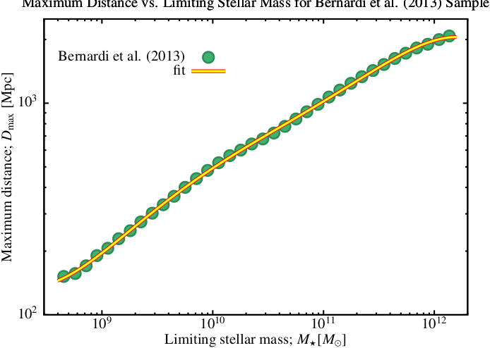
Fig. 8 The maximum distance at which a galaxy of given stellar mass can be detected in the sample of Bernardi et al. (2013). Points show the results obtained from data provided by Bernardi, while the lines shows a polynomial fit to these results (given in eqn. (21)).

surveyGeometryCaputi2011UKIDSSUDS

A survey geometry class which implements the UKIDSS UDS survey used by Caputi et al. (2011). The survey window function is determined from the set of galaxy positions provided by Caputi (private communication), by finding a suitable bounding box and then cutting out empty regions (corresponding to regions that were removed around bright stars). A set of random points are then found within this mask and are used to find the Fourier transform of the survey volume.

To estimate the depth of the Caputi et al. (2011) sample as a function of galaxy stellar mass we make use of semi-analytic models in the Millennium Database. Specifically, we use the SAM of Guo et al. (2011) and Henriques et al. (2012) specifically the Guo2010a..MR and Henriques2012a.wmap1.BC03_001 tables in the Millennium Database. For each snapshot in the database, we extract the stellar masses and observed-frame IRAC 4.5\(\mu\)m apparent magnitudes (including dust extinction), and determine the median apparent magnitude as a function of stellar mass. Using the limiting apparent magnitude of the Caputi et al. (2011) sample, \(i_{4.5}=24\), we infer the corresponding absolute magnitude at each redshift and, using our derived apparent magnitude–stellar mass relation, infer the corresponding stellar mass.

The end result of this procedure is the limiting stellar mass as a function of redshift, accounting for k-corrections, evolution, and the effects of dust. Figure 9 shows the resulting relation between stellar mass and the maximum redshift at which such a galaxy would be included in the sample. Points indicate measurements from the SAM, while the line shows a polynomial fit:

(22)\[z(M_\star) = -56.247 + 5.881 m,\]

where \(m= \log_{10}(M_\star/\mathrm{M}_\odot)\). We use this polynomial fit to determine the depth of the sample as a function of stellar mass.

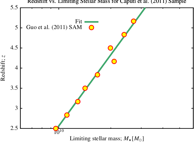
Fig. 9 The maximum redshift at which a galaxy of given stellar mass can be detected in the sample of Caputi et al. (2011). Points show the results obtained using the Henriques et al. (2012) model from the Millennium Database, while the lines shows a polynomial fit to these results (given in eqn. (22)).

Parameters

• [redshiftBin] — The redshift bin (0, 1, or 2) of the Caputi et al. (2011) to use.

surveyGeometryCombined

Implements a survey geometry which combines multiple other surveys.

surveyGeometryDavidzon2013VIPERS

A survey geometry class that describes the survey geometry of Davidzon et al. (2013).

For the angular mask, we make use of mangle polygon files provided by I. Davidzon (private communication) corresponding to the VIPERS fields. The solid angle of each mask is computed using the mangle harmonize command.

To determine the depth as a function of stellar mass, we make use of the tabulated mass function, \(\phi\), and number of galaxies per bin, \(N\), supplied by I. Davidzon (private communication). The effective volume of each bin is found as \(V_i = N_i/f_\mathrm{complete}\phi_i\Delta\log_{10}M_\star\), where \(\Delta\log_{10}M_\star\) is the width of the bin, and \(f_\mathrm{complete}\) is the completeness of the survey, estimated to be approximately 40% (Guzzo et al., 2014). These volumes are converted to maximum distances in each field using the survey solid angle. The resulting mass vs. distance relation in each field is fit with a \(1^\mathrm{st}\)-order polynomial in log-log space over the range where the maximum volume is limited by the survey depth and not by the imposed upper limit to redshift. Figure 10 shows the resulting relation between stellar mass and the maximum distance at which such a galaxy would be included in the sample. Points indicate results from VIPERS, while the lines show polynomial fits:

(23)\[\begin{split}\log_{10} \left[ {D_\mathrm{max}(M_\star) \over \hbox{Mpc}}\right] = \left\{ \begin{array}{ll} 3.207 + 0.0124m & 0.5 < z < 0.6 \\ 3.148 + 0.0268m & 0.6 < z < 0.8 \\ 3.207 + 0.0273m & 0.8 < z < 1.0 \end{array} \right.\end{split}\]

where \(m= \log_{10}(M_\star/\mathrm{M}_\odot)\). We use this polynomial fit to determine the depth of the sample as a function of stellar mass.

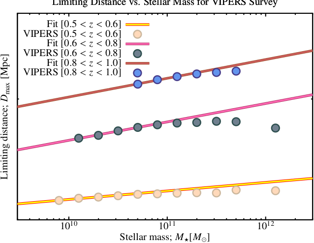
Fig. 10 The maximum distance at which a galaxy of given stellar mass can be detected in the sample of Davidzon et al. (2013). Points show the results obtained from data provided by Davidzon, while the lines shows a polynomial fit to these results (given in eqn. (23)). Note that at high masses the distance is limited by the imposed upper limit—the polynomial fit does not consider these points.

Parameters

• [redshiftBin] — The redshift bin (0, 1, 2) of the Davidzon et al. (2013) mass function to use.

surveyGeometryFullSky

Implements a survey geometry covering the full sky over a specified distance or redshift range. The survey volume is bounded by [redshiftMinimum] and [redshiftMaximum], with all sky positions included, making this suitable for theoretical or volume-limited analyses without angular masking.

Parameters

• [redshiftMinimum] (default 0.0d0) — The minimum redshift of the full-sky survey volume; sources below this redshift are excluded from the survey sample.

• [redshiftMaximum] (default huge(1.0d0)) — The maximum redshift of the full-sky survey volume; sources above this redshift are excluded from the survey sample.

surveyGeometryGunawardhana2013SDSS

Implements the geometry of the SDSS survey of Gunawardhana et al. (2013).

surveyGeometryHearin2014SDSS

Implements the survey geometry of the SDSS sample used by Hearin et al. (2014).

surveyGeometryKelvin2014GAMAnear

Implements the geometry of the GAMAnear survey of Kelvin et al. (2014).

surveyGeometryLiWhite2009SDSS

A survey geometry class that describes the survey geometry of Li and White (2009).

For the angular mask, we make use of the catalog of random points within the survey footprint provided by the NYU-VAGCfootnoteSpecifically, https://zenodo.org/records/10257229/files/lss_random-0.dr72.dat (which is a copy of the dataset originally found at the, now defunct, URL http://sdss.physics.nyu.edu/lss/dr72/random/lss_random-0.dr72.dat). (Blanton et al. 2005; see also Adelman-McCarthy et al. (2008), Padmanabhan et al. (2008)). Li and White (2009) consider only the main, contiguous region and so we keep only those points which satisfy RA\(>100^\circ\), RA\(<300^\circ\), and RA\(<247^\circ\) or \(\delta< 51^\circ\). When the survey window function is needed, these points are used to determine which elements of a 3D grid fall within the window function.

To estimate the depth of the Li and White (2009) sample as a function of galaxy stellar mass we make use of semi-analytic models in the Millennium Database. Specifically, we use the SAM of De Lucia and Blaizot (2007; specifically the millimil..DeLucia2006a and millimil..DeLucia2006a_sdss2mass tables in the Millennium Database). For each snapshot in the database, we extract the stellar masses and observed-frame SDSS r-band absolute magnitudes (including dust extinction), and determine the median absolute magnitude as a function of stellar mass. Using the limiting apparent magnitude of the Li and White (2009) sample, \(r=17.6\), we infer the corresponding absolute magnitude at each redshift and, using our derived absolute magnitude–stellar mass relation, infer the corresponding stellar mass.

The end result of this procedure is the limiting stellar mass as a function of redshift, accounting for k-corrections, evolution, and the effects of dust. Figure 11 shows the resulting relation between stellar mass and the maximum redshift at which such a galaxy would be included in the sample. Points indicate measurements from the SAM, while the line shows a polynomial fit:

(24)\[\begin{split}z(M_\star) & = -5.950 + 2.638 m - 0.4211 m^2 \nonumber \\ & + 2.852\times 10^{-2} m^3 - 6.783 \times 10^{-4} m^4,\end{split}\]

where \(m= \log_{10}(M_\star/\mathrm{M}_\odot)\). We use this polynomial fit to determine the depth of the sample as a function of stellar mass. We adopt a solid angle of \(2.1901993\) sr (Percival et al., 2007) for the sample.

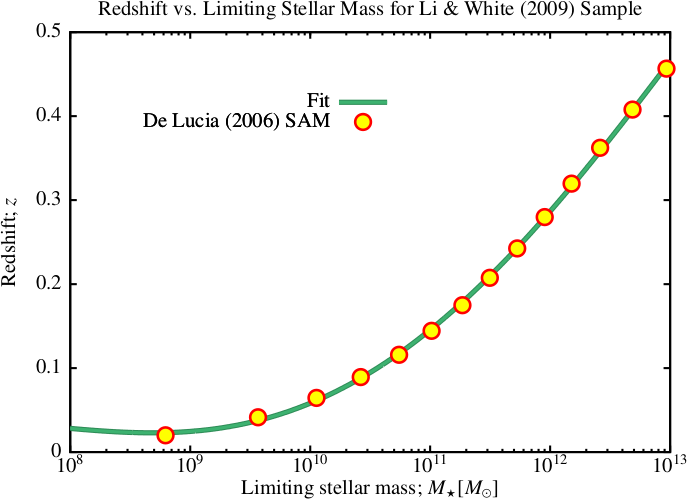
Fig. 11 The maximum redshift at which a galaxy of given stellar mass can be detected in the sample of Li and White (2009). Points show the results obtained using the De Lucia and Blaizot (2007) model from the Millennium Database, while the lines shows a polynomial fit to these results (given in eqn. (24)).

(Default implementation)

Parameters

• [redshiftMinimum] (default 0.0d0) — The minimum redshift of the Li and White (2009) survey volume; sources below this redshift are excluded from the survey sample.

• [redshiftMaximum] (default huge(1.0d0)) — The maximum redshift of the Li and White (2009) survey volume; sources above this redshift are excluded from the survey sample.

surveyGeometryLocalGroupClassical

Implements a survey geometry corresponding to the detectability of classical Local Group satellite galaxies, defined by mangle polygon sky coverage. The maximum detection distance is set by [distanceMaximumSurvey], and a stellar mass threshold [massThreshold] separates classical from ultra-faint satellites.

Parameters

• [distanceMaximumSurvey] (default 300.0d-3) — The maximum distance for the sample of classical Local Group galaxies.

• [massThreshold] (default 1.0d5) — The minimum stellar mass for a classical Local Group dwarf galaxy.

surveyGeometryLocalGroupDES

Implements the angular footprint and maximum detection distance of the Dark Energy Survey (DES) as applied to Local Group dwarf galaxy searches. The survey volume is defined by mangle polygon files, with the maximum survey distance set by [distanceMaximumSurvey].

Parameters

• [distanceMaximumSurvey] (default 300.0d-3) — The maximum distance at which galaxies are to be included in the survey.

surveyGeometryLocalGroupSDSS

Implements the angular footprint of the SDSS survey adapted for Local Group dwarf galaxy detectability, with the maximum survey depth set by [distanceMaximumSurvey]. This geometry is used to model the detection volume of faint dwarf galaxies in the nearby Universe.

Parameters

• [distanceMaximumSurvey] (default 300.0d-3) — The maximum distance at which galaxies are to be included in the survey.

surveyGeometryMangle

Implements an abstract survey geometry using mangle polygons.

Methods

• mangleDirectory — Return the directory containing mangle files for this survey geometry.

• mangleFiles — Return array of mangle filenames for this survey geometry.

• initialize — Initialize an instance of the mangle survey geometry class.

surveyGeometryMartin2010ALFALFA

A survey geometry class that describes the survey geometry of Martin et al. (2010).

For the angular mask we use the three disjoint regions defined by 07\(^\mathrm{h}\)30\(^\mathrm{m}\) \(<\) R.A. \(<\) 16\(^\mathrm{h}\)30\(^\mathrm{m}\), +04\(^\circ\) \(<\) decl. \(<\) +16\(^\circ\), and +24\(^\circ\) \(<\) decl. \(<\) +28\(^\circ\) and 22\(^\mathrm{h}\) \(<\) R.A. \(<\) 03\(^\mathrm{h}\), +14\(^\circ\) \(<\) decl. \(<\) +16\(^\circ\), and +24\(^\circ\) \(<\) decl. \(<\) +32\(^\circ\) corresponding to the sample of Martin et al. (2010). When the survey window function is needed we generate randomly distributed points within this angular mask and out to the survey depth. These points are used to determine which elements of a 3D grid fall within the window function.

To estimate the depth of the Martin et al. (2010) sample as a function of galaxy HI mass we first infer the median line width corresponding to that mass. To do so, we have fit the median line width-mass relation from the \(\alpha.40\) sample with power-law function as shown in Fig. 12. We find that the median line width can be approximated by

(25)\[\log_{10} (W_\mathrm{50}/\hbox{km s}^{-1}) = c_0 + c_1 \log_10(M_\mathrm{HI}/\mathrm{M}_\odot),\]

with \(c_0=-0.770\) and \(c_1=0.315\). Given the line width, the corresponding integrated flux limit, \(S_\mathrm{int}\), for a signal-to-noise of \(6.5\) is inferred using equation (A1) of Haynes et al. (2011). Finally, this integrated flux limit is converted to maximum distance at which the source could be detected using the expression given in the text of section 2.2 of Martin et al. (2010):

\[M_\mathrm{HI} = 2.356\times10^5 \left({D\over \hbox{Mpc}}\right)^2 \left({S_\mathrm{int}\over\hbox{Jy km s}^{-1}}\right).\]

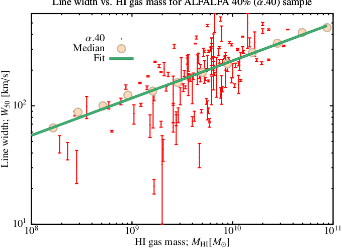
Fig. 12 HI line width vs. HI mass as measured from the \(\alpha.40\) survey of Martin et al. (2010). Red points with error bars show individual measurements, while the larger circles indicate the running median of these data. The green line is a power-law fit to the running median as described in eqn. ((25)).

surveyGeometryMonteroDorta2009SDSS

Implements the geometry of the SDSS survey as used by Montero-Dorta and Prada (2009) for their luminosity function measurements. The effective survey volume is defined by redshift limits [redshiftMinimum] and [redshiftMaximum] and apparent magnitude limits in a specified photometric [band].

Parameters

• [band] — The band for which the survey geometry should be computed.

surveyGeometryMoustakas2013PRIMUS

A survey geometry class that describes the survey geometry of Moustakas et al. (2013).

For the angular mask, we make use of mangle polygon files provided by J. Moustakas (private communication) corresponding to the give PRIMUS fields. The solid angle of each mask is computed using the mangle harmonize command.

To determine the depth as a function of stellar mass, we make use of completeness limits for “All” galaxies given in Table 2 of Moustakas et al. (2013). These are fit, for each field with a second order polynomial to give the limiting redshift as a function of stellar mass. Figure 13 shows the resulting relation between stellar mass and the maximum redshift at which such a galaxy would be included in the sample. Points indicate results from Moustakas et al. (2013), while the line shows a polynomial fits:

(26)\[\begin{split}z_\mathrm{max}(M_\star) = +3.51+m(-0.941+m(+0.0651)) & \hbox{COSMOS} \\ z_\mathrm{max}(M_\star) = +2.46+m(-0.730+m(+0.0542)) & \hbox{XMM-SXDS} \\ z_\mathrm{max}(M_\star) = -3.60+m(+0.500+m(-0.0078)) & \hbox{XMM-CFHTLS} \\ z_\mathrm{max}(M_\star) = +5.87+m(-1.528+m(+0.0982)) & \hbox{CDFS} \\ z_\mathrm{max}(M_\star) = +6.87+m(-1.656+m(+0.1003)) & \hbox{ELAIS-S1}\end{split}\]

where \(m= \log_{10}(M_\star/\mathrm{M}_\odot)\). We use this polynomial fit to determine the depth of the sample as a function of stellar mass.

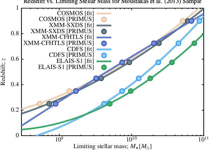
Fig. 13 The maximum distance at which a galaxy of given stellar mass can be detected in the sample of Moustakas et al. (2013). Points show the results obtained from completeness limit data taken from Table 2 of Moustakas et al. (2013), while the lines shows a polynomial fit to these results (given in eqn. (26)).

Parameters

• [redshiftBin] — The redshift bin (0, 1, 2, 3, 4, 5, or 5) of the Moustakas et al. (2013) mass function to use.

surveyGeometryMuzzin2013ULTRAVISTA

A survey geometry class that describes the survey geometry of Muzzin et al. (2013).

For the angular mask, we generate a mangle polygon file, by first defining a rectangle encompassing the bounds of the ULTRAVISTA field (\(149.373^\circ < \alpha < 150.779^\circ\) and \(1.604^\circ < \delta < 2.81^\circ\)). From this rectangle, we then remove circles of radii \(75^{\prime\prime}\) around bright stars (i.e. those bright than 10\(^\mathrm{th}\) and \(8^\mathrm{th}\) magnitudes in the USNO and 2MASS star lists respectively) and radii \(30^{\prime\prime}\) around medium stars (i.e. those bright than \(13^\mathrm{th}\) and \(10.5^\mathrm{th}\) magnitudes in the USNO and 2MASS star lists respectively). Finally, we mask regions of one detector for which 75% of pixels are dead by clipping pixels with weights below \(0.02\) in the K\(_\mathrm{s}\)-band weight map. These choices match those made in the ULTRAVISTA survey (A. Muzzin, private communication). The solid angle of each mask is computed using the mangle harmonize command.

To determine the depth as a function of stellar mass, we simply fit the tabulated relations provided by the ULTRAVISTA survey:

(27)\[z_\mathrm{max}(M_\star) = {-8364.45 + m (4331.82 + m (-896.596 + m (92.6999 + m (-4.78750 + m (0.0988215))))) \over 1 - \exp[(m-11.24)/0.02] }\]

where \(m= \log_{10}(M_\star/\mathrm{M}_\odot)\).

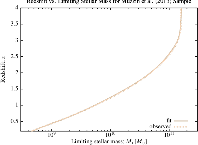
Fig. 14 The maximum distance at which a galaxy of given stellar mass can be detected in the sample of Muzzin et al. (2013). The dotted line shows the results obtained from the ULTRAVISTA survey (Muzzin et al., 2013), while the solid line shows the polynomial fit to these results (given in eqn. (27)).

Parameters

• [redshiftBin] — The redshift bin (0, 1, 2, 3, 4, 5, or 6) of the Muzzin et al. (2013) mass function to use.

surveyGeometryRandomPoints

Implements survey geometries defined by random points.

Methods

• randomsInitialize — Initialize arrays of random points to define the survey angular geometry.

surveyGeometryTomczak2014ZFOURGE

A survey geometry class that describes the survey geometry of Tomczak et al. (2014).

For the angular mask, we make use of mangle polygon files constructed by hand using vertices matched approximately to the distribution of galaxies in the survey (positions of which were provided by R. Quadri; private communication). The solid angle of each mask is computed using the mangle harmonize command.

To determine the depth as a function of stellar mass, we make use of the tabulated mass completeness limits as a function of redshift for ZFOURGE and NMBS fields provided by R. Quadri (private communication). These are fit with fourth-order polynomials. Figure 15 shows the resulting relation between stellar mass and the maximum redshift at which such a galaxy would be included in the sample. Dotted lines indicate the tabulated result from ZFOURGE, while the lines show polynomial fits:

(28)\[\begin{split}z_\mathrm{max}(M_\star) = \left\{ \begin{array}{ll} -114.66+m*(45.901+m*(-6.1617+m*(0.27822))) & \hbox{ZFOURGE fields} \\ -58.483+m*(20.250+m*(-2.3563+m*(0.092705))) & \hbox{NMBS fields} \end{array} \right.\end{split}\]

where \(m= \log_{10}(M_\star/\mathrm{M}_\odot)\). We use this polynomial fit to determine the depth of the sample as a function of stellar mass.

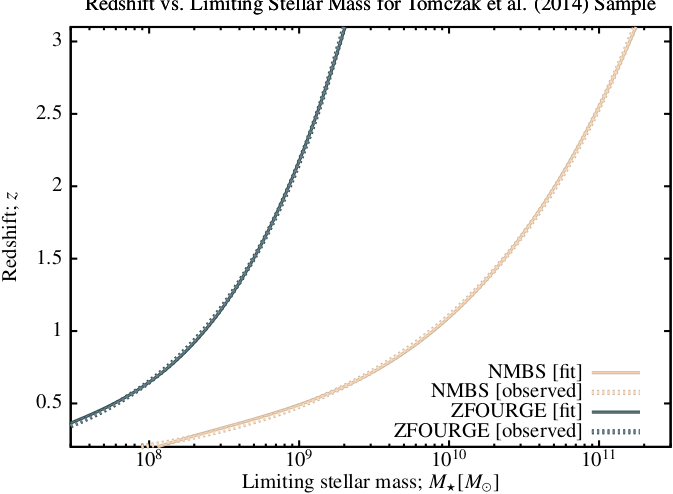
Fig. 15 The maximum redshift at which a galaxy of given stellar mass can be detected in the sample of Tomczak et al. (2014). Points show the results obtained from data provided by Davidzon, while the lines shows a polynomial fit to these results (given in eqn. (28)).

Parameters

• [redshiftBin] — The redshift bin (0, 1, 2, 3, 4, 5, 6, or 7) of the Tomczak et al. (2014) mass function to use.