Tutorial 1: Galacticus as a cosmology calculator

Galacticus is a semi-analytic model of galaxy formation. Its physics engine — every functionClass of the Fortran code, from cosmology through dark-matter halos to stellar populations — is exposed to Python through the libgalacticus shared library, so you can use the same implementations that power full galaxy formation runs as building blocks in your own scripts and notebooks.

This first tutorial introduces the two ideas you need:

1. Objects are built from parameter values and other objects. Galacticus is organized around abstract classes (cosmologyParameters, cosmologyFunctions, transferFunction, …), each with interchangeable implementations. In Python you instantiate an implementation by calling its constructor with plain values and previously-constructed objects.

2. Methods are ordinary Python calls returning floats, numpy arrays, or tuples.

Here we drive the cosmology classes: expansion history, times, densities, and distances.

Units (Galacticus conventions): masses in \(M_\odot\), times in Gyr, distances in Mpc, \(H_0\) in km/s/Mpc, wavenumbers in comoving Mpc\(^{-1}\).

Setup

Load the library. If you built Galacticus from source with make GALACTICUS_BUILD_OPTION=lib libgalacticus.so and are running this notebook from the tutorials/ folder of the source tree, this cell works as-is; otherwise point GALACTICUS_LIBRARY_PATH at the directory containing the galacticus/ folder of the binary distribution.

Troubleshooting — ``OSError: … version ‘GCC_x.y.0’ not found``. libgalacticus.so links against your compiler’s C++/GCC runtime (libstdc++.so.6, libgcc_s.so.1); if your Python environment loads older copies, importing galacticus fails with, e.g., libgcc_s.so.1: version `GCC_14.0.0' not found. In a shell an LD_PRELOAD=/path/to/compiler/lib64/libstdc++.so.6 python3 ... fixes it, but that cannot be done from a notebook cell: the linker reads LD_PRELOAD only at process startup, and the kernel has already loaded the old libraries before this cell runs. Instead, create a dedicated Jupyter kernel whose kernel.json sets LD_PRELOAD (to the correct libgcc_s.so.1 and libstdc++.so.6) in its env block, and select it via Kernel → Change Kernel. See the “Troubleshooting” section of `README.md <README.md>`__ for the exact kernel.json.

import os, sys

# Locate the Galacticus library interface. Two supported layouts:
#  * a Galacticus source tree built with
#      make GALACTICUS_BUILD_OPTION=lib libgalacticus.so
#    (galacticus.py at the tree root, the library under galacticus/lib/);
#  * an unpacked binary distribution (the `galacticus/` folder from
#    libgalacticus.tar.bz2, with python/ and lib/ inside it).
# Set GALACTICUS_LIBRARY_PATH to the directory CONTAINING the `galacticus/`
# folder if the auto-detection below does not fit your setup.
root = os.environ.get('GALACTICUS_LIBRARY_PATH',
                      os.path.abspath(os.path.join(os.getcwd(), os.pardir)))
os.chdir(root)   # galacticus.py loads galacticus/lib/libgalacticus.so relative to here
for candidate in (root, os.path.join(root, 'galacticus', 'python')):
    if os.path.exists(os.path.join(candidate, 'galacticus.py')):
        sys.path.insert(0, candidate)
        break
else:
    raise RuntimeError(f"galacticus.py not found under {root} - build the library "
                       "(make GALACTICUS_BUILD_OPTION=lib libgalacticus.so) or set "
                       "GALACTICUS_LIBRARY_PATH")

import numpy as np
import matplotlib.pyplot as plt
import galacticus
print("Galacticus library interface loaded.")

Galacticus library interface loaded.

plt.rcParams.update({'figure.figsize': (7.0, 4.5), 'font.size': 11,
                     'axes.grid': True, 'grid.alpha': 0.3})

Cosmological parameters

The cosmologyParametersSimple implementation holds a flat set of parameters: \(\Omega_\mathrm{M}\), \(\Omega_\mathrm{b}\), \(\Omega_\Lambda\), \(T_\mathrm{CMB}\) [K], and \(H_0\) [km/s/Mpc].

cosmologyParameters = galacticus.cosmologyParametersSimple(
    OmegaMatter    = 0.3,
    OmegaBaryon    = 0.045,
    OmegaDarkEnergy= 0.7,
    temperatureCMB = 2.78,
    HubbleConstant = 70.0,
)
print(f"Omega_M          = {cosmologyParameters.OmegaMatter():.3f}")
print(f"Omega_b          = {cosmologyParameters.OmegaBaryon():.3f}")
print(f"Omega_DE         = {cosmologyParameters.OmegaDarkEnergy():.3f}")
print(f"Omega_curvature  = {cosmologyParameters.OmegaCurvature():.3f}")
print(f"H_0              = {cosmologyParameters.HubbleConstant():.1f} km/s/Mpc")
print(f"critical density = {cosmologyParameters.densityCritical():.4e} Msun/Mpc^3")

Omega_M          = 0.300
Omega_b          = 0.045
Omega_DE         = 0.700
Omega_curvature  = 0.000
H_0              = 70.0 km/s/Mpc
critical density = 1.3598e+11 Msun/Mpc^3

Expansion history

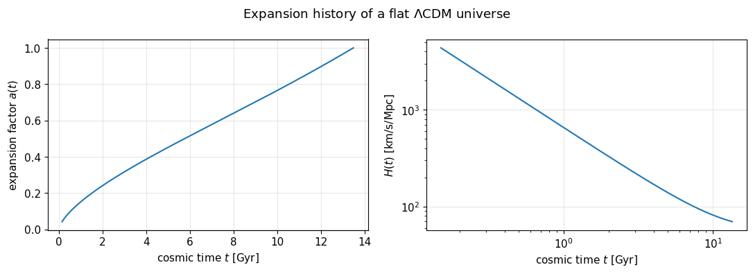
cosmologyFunctionsMatterLambda solves the Friedmann equation for a matter + cosmological-constant universe. It is constructed from the parameters object — this dependency-injection pattern is how every Galacticus object graph is assembled.

cosmologyFunctions = galacticus.cosmologyFunctionsMatterLambda(cosmologyParameters)

ageToday = cosmologyFunctions.cosmicTime(1.0)      # time at expansion factor a=1
print(f"Age of the Universe today : {ageToday:.3f} Gyr")
for z in (0.5, 2.0, 6.0, 20.0):
    a = cosmologyFunctions.expansionFactorFromRedshift(z)
    t = cosmologyFunctions.cosmicTime(a)
    print(f"  z = {z:5.1f}  ->  a = {a:.4f},  t = {t:6.3f} Gyr,"
          f"  H = {cosmologyFunctions.hubbleParameterEpochal(time=t):7.1f} km/s/Mpc")

Age of the Universe today : 13.467 Gyr
  z =   0.5  ->  a = 0.6667,  t =  8.426 Gyr,  H =    91.6 km/s/Mpc
  z =   2.0  ->  a = 0.3333,  t =  3.227 Gyr,  H =   207.7 km/s/Mpc
  z =   6.0  ->  a = 0.1429,  t =  0.917 Gyr,  H =   712.5 km/s/Mpc
  z =  20.0  ->  a = 0.0476,  t =  0.177 Gyr,  H =  3690.1 km/s/Mpc

# Expansion factor and Hubble rate through cosmic time.
times = np.linspace(0.15, ageToday, 300)
a     = np.array([cosmologyFunctions.expansionFactor(t)                for t in times])
H     = np.array([cosmologyFunctions.hubbleParameterEpochal(time=t)   for t in times])

fig, axes = plt.subplots(1, 2, figsize=(11, 4))
axes[0].plot(times, a)
axes[0].set_xlabel('cosmic time $t$ [Gyr]'); axes[0].set_ylabel('expansion factor $a(t)$')
axes[1].loglog(times, H)
axes[1].set_xlabel('cosmic time $t$ [Gyr]'); axes[1].set_ylabel('$H(t)$ [km/s/Mpc]')
fig.suptitle('Expansion history of a flat $\\Lambda$CDM universe')
fig.tight_layout()
plt.show()

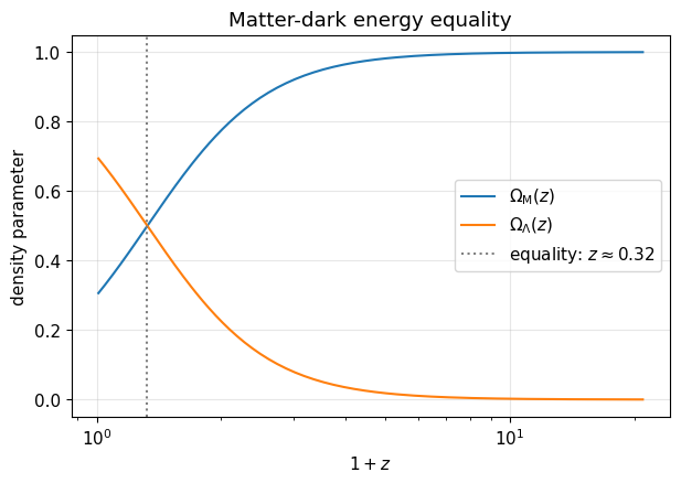
The changing energy budget

\(\Omega_\mathrm{M}(t)\) and \(\Omega_\Lambda(t)\) trade places around \(z \sim 0.3\): matter domination gives way to dark-energy domination, which is why structure growth slows at late times (Tutorial 2).

zGrid = np.logspace(-2, 1.3, 200)
tGrid = np.array([cosmologyFunctions.cosmicTime(
                      cosmologyFunctions.expansionFactorFromRedshift(z)) for z in zGrid])
OmegaM  = np.array([cosmologyFunctions.omegaMatterEpochal   (time=t) for t in tGrid])
OmegaDE = np.array([cosmologyFunctions.omegaDarkEnergyEpochal(time=t) for t in tGrid])

plt.semilogx(1.0+zGrid, OmegaM , label='$\\Omega_\\mathrm{M}(z)$')
plt.semilogx(1.0+zGrid, OmegaDE, label='$\\Omega_\\Lambda(z)$')
zEq = zGrid[np.argmin(np.abs(OmegaM-OmegaDE))]
plt.axvline(1.0+zEq, color='gray', ls=':', label=f'equality: $z\\approx{zEq:.2f}$')
plt.xlabel('$1+z$'); plt.ylabel('density parameter'); plt.legend()
plt.title('Matter-dark energy equality')
plt.show()

Distances

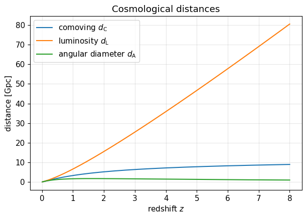
Galacticus’s distance functions take cosmic time as their argument; use expansionFactorFromRedshift + cosmicTime to convert from redshift. The familiar textbook relations between comoving, luminosity, and angular diameter distances hold: \(d_\mathrm{L} = (1+z)\,d_\mathrm{C}\) and \(d_\mathrm{A} = d_\mathrm{C}/(1+z)\) in a flat universe.

zGrid = np.linspace(0.01, 8.0, 200)
tGrid = np.array([cosmologyFunctions.cosmicTime(
                      cosmologyFunctions.expansionFactorFromRedshift(z)) for z in zGrid])
dC = np.array([cosmologyFunctions.distanceComoving  (t) for t in tGrid])
dL = np.array([cosmologyFunctions.distanceLuminosity(t) for t in tGrid])
dA = np.array([cosmologyFunctions.distanceAngular   (t) for t in tGrid])

plt.plot(zGrid, dC/1.0e3, label='comoving $d_\\mathrm{C}$')
plt.plot(zGrid, dL/1.0e3, label='luminosity $d_\\mathrm{L}$')
plt.plot(zGrid, dA/1.0e3, label='angular diameter $d_\\mathrm{A}$')
plt.xlabel('redshift $z$'); plt.ylabel('distance [Gpc]'); plt.legend()
plt.title('Cosmological distances')
plt.show()

# Internal consistency checks.
i = np.argmin(np.abs(zGrid-2.0)); z = zGrid[i]
assert np.isclose(dL[i], (1.0+z)   *dC[i], rtol=1.0e-6)
assert np.isclose(dA[i],  dC[i]/(1.0+z)  , rtol=1.0e-6)
print(f"d_L=(1+z)d_C and d_A=d_C/(1+z) verified at z={z:.2f}")

d_L=(1+z)d_C and d_A=d_C/(1+z) verified at z=2.02

Comparing cosmologies

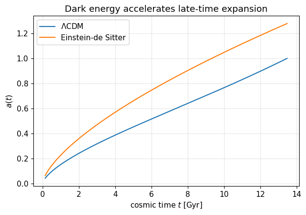
Because objects are cheap to construct, comparing cosmologies is a two-line affair. Here: our fiducial flat \(\Lambda\)CDM against an Einstein-de Sitter universe (\(\Omega_\mathrm{M}=1\)).

cosmologyParametersEdS = galacticus.cosmologyParametersSimple(1.0, 0.045, 0.0, 2.78, 70.0)
cosmologyFunctionsEdS  = galacticus.cosmologyFunctionsMatterLambda(cosmologyParametersEdS)

print(f"Age of the Universe:  LCDM = {cosmologyFunctions.cosmicTime(1.0):6.3f} Gyr,"
      f"  EdS = {cosmologyFunctionsEdS.cosmicTime(1.0):6.3f} Gyr")

times = np.linspace(0.15, ageToday, 200)
for label, cf in (('$\\Lambda$CDM', cosmologyFunctions), ('Einstein-de Sitter', cosmologyFunctionsEdS)):
    plt.plot(times, [cf.expansionFactor(t) for t in times], label=label)
plt.xlabel('cosmic time $t$ [Gyr]'); plt.ylabel('$a(t)$'); plt.legend()
plt.title('Dark energy accelerates late-time expansion')
plt.show()

Age of the Universe:  LCDM = 13.467 Gyr,  EdS =  9.312 Gyr

Where next

• Tutorial 2 builds the linear matter power spectrum from these same objects — including warm-dark-matter variants.

• Tutorial 3 computes halo mass functions across cosmic time.

• Tutorial 4 shows Galacticus calling back into your Python functions.