Tutorial 6: Stellar populations

Everything a semi-analytic model knows about stars enters through a small set of functionClass families: the initial mass function (IMF), stellar astrophysics (lifetimes, remnant and ejected masses, yields), and the supernova rates built on top of them. All are driven directly from Python here.

This tutorial needs the Galacticus datasets (the stellar-properties compilation) — see the setup cell.

import os, sys

# Locate the Galacticus library interface (see Tutorial 1 for details).
root = os.environ.get('GALACTICUS_LIBRARY_PATH',
                      os.path.abspath(os.path.join(os.getcwd(), os.pardir)))
os.chdir(root)   # galacticus.py loads galacticus/lib/libgalacticus.so relative to here
for candidate in (root, os.path.join(root, 'galacticus', 'python')):
    if os.path.exists(os.path.join(candidate, 'galacticus.py')):
        sys.path.insert(0, candidate)
        break
else:
    raise RuntimeError(f"galacticus.py not found under {root} - build the library "
                       "(make GALACTICUS_BUILD_OPTION=lib libgalacticus.so) or set "
                       "GALACTICUS_LIBRARY_PATH")

# This tutorial also reads Galacticus's static datasets (the stellar
# properties compilation): clone https://github.com/galacticusorg/datasets
# and point GALACTICUS_DATA_PATH at it.
if 'GALACTICUS_DATA_PATH' not in os.environ:
    raise RuntimeError("set GALACTICUS_DATA_PATH to a clone of "
                       "https://github.com/galacticusorg/datasets")

import numpy as np
if not hasattr(np, 'trapezoid'):        # np.trapezoid is NumPy >= 2.0;
    np.trapezoid = np.trapz             # fall back to the pre-2.0 name.
import matplotlib.pyplot as plt
import galacticus
print("Galacticus library interface loaded.")

Galacticus library interface loaded.

plt.rcParams.update({'figure.figsize': (7.0, 4.5), 'font.size': 11,
                     'axes.grid': True, 'grid.alpha': 0.3})

Initial mass functions

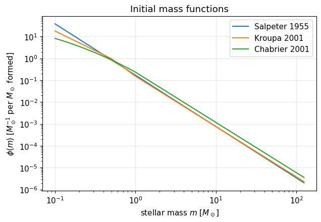
phi(m) returns \(\phi(m) = \mathrm{d}N/\mathrm{d}m\) per unit stellar mass formed — each IMF is normalized so \(\int m\,\phi(m)\,\mathrm{d}m = 1\). We compare the three classics; the Chabrier (2001) parameters shown are Galacticus’s defaults (lognormal below \(1\,M_\odot\), power law above).

imfSalpeter = galacticus.initialMassFunctionSalpeter1955()
imfKroupa   = galacticus.initialMassFunctionKroupa2001()
imfChabrier = galacticus.initialMassFunctionChabrier2001(
    massLower=0.1, massTransition=1.0, massUpper=125.0,
    exponent=-2.3, massCharacteristic=0.08, sigma=0.69)
imfs = (('Salpeter 1955', imfSalpeter), ('Kroupa 2001', imfKroupa),
        ('Chabrier 2001', imfChabrier))

masses = np.logspace(-1, np.log10(124.0), 300)
for label, imf in imfs:
    plt.loglog(masses, [imf.phi(m) for m in masses], label=label)
plt.xlabel('stellar mass $m$ [$M_\\odot$]')
plt.ylabel('$\\phi(m)$ [$M_\\odot^{-1}$ per $M_\\odot$ formed]')
plt.legend(); plt.title('Initial mass functions')
plt.show()

# Verify the unit mass normalization by direct integration of phi.
for label, imf in imfs:
    grid = np.logspace(np.log10(imf.massMinimum()), np.log10(imf.massMaximum()), 8001)
    norm = np.trapezoid([m*imf.phi(m) for m in grid], grid)
    print(f"{label:14s}: integral of m*phi(m) dm = {norm:.4f}")

Salpeter 1955 : integral of m*phi(m) dm = 1.0000
Kroupa 2001   : integral of m*phi(m) dm = 1.0000
Chabrier 2001 : integral of m*phi(m) dm = 1.0000

Astrophysically the differences live at the extremes: Salpeter’s unbroken power law puts far more mass into (invisible, long-lived) low-mass stars, while the turned-over IMFs put relatively more into the massive stars that drive supernova feedback. numberCumulative integrates the count — here, core-collapse supernova progenitors (\(8\)–\(125\,M_\odot\)) per solar mass of stars formed:

for label, imf in imfs:
    print(f"{label:14s}: {imf.numberCumulative(8.0, 125.0):.5f} SN II progenitors per Msun formed")

Salpeter 1955 : 0.00743 SN II progenitors per Msun formed
Kroupa 2001   : 0.00761 SN II progenitors per Msun formed
Chabrier 2001 : 0.01179 SN II progenitors per Msun formed

Stellar astrophysics: lifetimes, remnants and yields

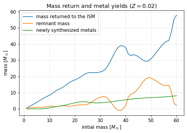
stellarAstrophysicsFile interpolates the standard compilation of stellar-evolution models shipped with Galacticus (the %DATASTATICPATH% token expands to the static datasets path). Three textbook results in three plots: the steep lifetime-mass relation and its weak metallicity dependence, the main-sequence turnoff mass as a clock, and how much of a star’s mass is returned to the interstellar medium.

stellarAstrophysics = galacticus.stellarAstrophysicsFile(
    "%DATASTATICPATH%/stellarAstrophysics/stellarPropertiesCompilationStandard.xml")

massGrid = np.logspace(0.0, 2.0, 60)
fig, axes = plt.subplots(1, 2, figsize=(11.5, 4.3))
for Z, color in ((0.0004, 'C0'), (0.004, 'C1'), (0.02, 'C2')):
    axes[0].loglog(massGrid, [stellarAstrophysics.lifetime(m, Z) for m in massGrid],
                   color=color, label=f'$Z={Z}$')
axes[0].set_xlabel('initial mass [$M_\\odot$]'); axes[0].set_ylabel('lifetime [Gyr]')
axes[0].legend(); axes[0].set_title('Stellar lifetimes')

ages = np.logspace(-2.5, 1.1, 60)
axes[1].loglog(ages, [stellarAstrophysics.massInitial(age, 0.02) for age in ages], color='C2')
axes[1].set_xlabel('population age [Gyr]'); axes[1].set_ylabel('turnoff mass [$M_\\odot$]')
axes[1].set_title('Main-sequence turnoff as a clock')
fig.tight_layout(); plt.show()

print(f"Solar-mass, solar-metallicity lifetime: "
      f"{stellarAstrophysics.lifetime(1.0, 0.02):.1f} Gyr")

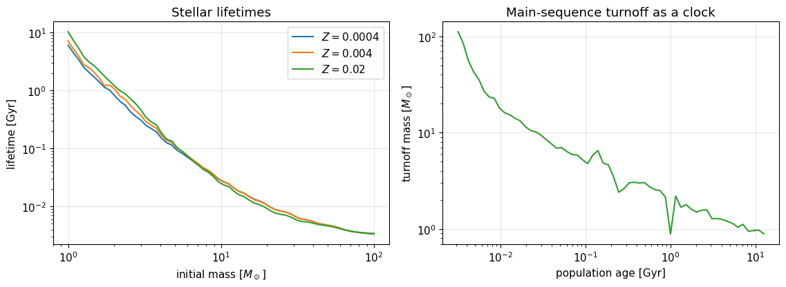
Solar-mass, solar-metallicity lifetime: 10.3 Gyr

massGrid = np.linspace(1.0, 60.0, 60)
ejected  = np.array([stellarAstrophysics.massEjected(m, 0.02) for m in massGrid])
yieldMetals = np.array([stellarAstrophysics.massYield(m, 0.02) for m in massGrid])
plt.plot(massGrid, ejected          , label='mass returned to the ISM')
plt.plot(massGrid, massGrid-ejected , label='remnant mass')
plt.plot(massGrid, yieldMetals      , label='newly synthesized metals')
plt.xlabel('initial mass [$M_\\odot$]'); plt.ylabel('mass [$M_\\odot$]')
plt.legend(); plt.title('Mass return and metal yields ($Z=0.02$)')
plt.show()

Type Ia supernova delay-time distribution

Type Ia supernovae trace old populations: after a minimum delay for the first white dwarfs to form, the rate falls off roughly as \(t^{-1}\). supernovaeTypeIaPowerLawDTDDifferential.number gives the cumulative number of SNe Ia per solar mass formed by a given population age (the \(2\times10^{-3}\,M_\odot^{-1}\) normalization and \(t^{-1}\) slope follow Maoz et al. 2012).

snIa = galacticus.supernovaeTypeIaPowerLawDTDDifferential(
    timeMinimum=0.04, exponent=-1.0, normalization=2.0e-3)
ages = np.logspace(-2, 1.13, 120)
number = np.array([snIa.number(imfChabrier, 1.0, age, 0.02) for age in ages])
plt.semilogx(ages, 1.0e3*number)
plt.axvline(0.04, color='gray', ls=':', label='minimum delay (40 Myr)')
plt.xlabel('population age [Gyr]')
plt.ylabel('cumulative SNe Ia per $10^3\\,M_\\odot$ formed')
plt.legend(); plt.title('A $t^{-1}$ Type Ia delay-time distribution')
plt.show()
print(f"SNe Ia per Msun formed within 10 Gyr: {snIa.number(imfChabrier, 1.0, 10.0, 0.02):.3e}")

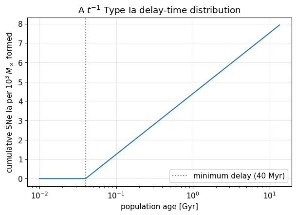
SNe Ia per Msun formed within 10 Gyr: 7.522e-03

What about full spectra?

Simple-stellar-population spectra (stellarPopulationSpectraFSPS) are exposed through the same interface, but constructing that class triggers, on first use, a download-compile-run of the FSPS package to tabulate the spectra — too heavy for a tutorial that executes in CI. If you have a Galacticus installation that has already built its FSPS tables, the class works from Python like any other; spectral evaluation per-wavelength additionally requires an abundances object, which the library interface does not yet construct from Python.

Where next

These classes are the atoms from which Galacticus builds its chemical evolution and feedback: stellarPopulationProperties integrates them over star-formation histories, and stellarFeedback turns them into energy injection. Combined with Tutorials 3 and 5, you now have the full chain from the power spectrum to the stars.