Tutorial 7: Survey geometries

Comparing a galaxy formation model against survey data means knowing exactly where the survey looked: its angular mask on the sky, and how far away a galaxy of given luminosity or mass remains detectable. In Galacticus this is the surveyGeometry class, used to compute \(V_\mathrm{max}\) weights for luminosity/mass functions and window functions for power-spectrum comparisons.

Highlights of this tutorial:

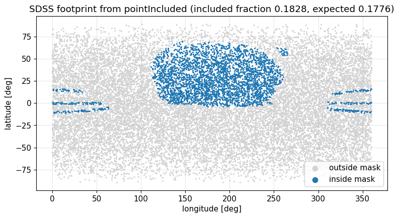
• the SDSS angular mask of Bernardi et al. (2013), driven through its mangle polygon representation — including reconstructing the survey footprint point by point;

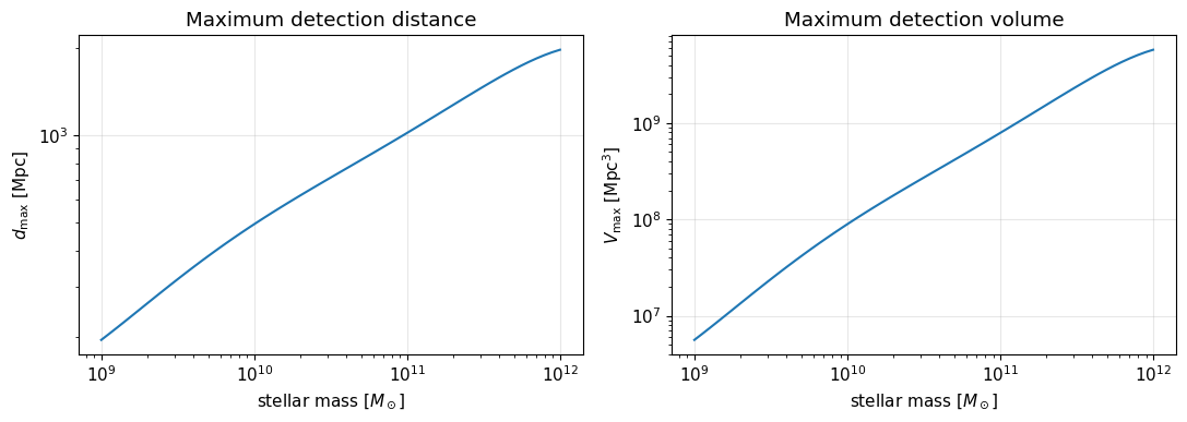
• \(V_\mathrm{max}(M)\), the workhorse of mass-function estimation;

• Fourier-space window functions on a 3D grid (computed by FFTW inside Galacticus, returned to Python as complex arrays), cross-validated against numpy’s FFT and the analytic expectation — for the full sky and for the real SDSS mask, Monte-Carlo sampled from its polygons;

• the payoff: convolving a theory power spectrum with a survey window, the operation at the heart of every P(k) comparison.

import os, sys

# Locate the Galacticus library interface (see Tutorial 1 for details).
root = os.environ.get('GALACTICUS_LIBRARY_PATH',
                      os.path.abspath(os.path.join(os.getcwd(), os.pardir)))
os.chdir(root)   # galacticus.py loads galacticus/lib/libgalacticus.so relative to here
for candidate in (root, os.path.join(root, 'galacticus', 'python')):
    if os.path.exists(os.path.join(candidate, 'galacticus.py')):
        sys.path.insert(0, candidate)
        break
else:
    raise RuntimeError(f"galacticus.py not found under {root} - build the library "
                       "(make GALACTICUS_BUILD_OPTION=lib libgalacticus.so) or set "
                       "GALACTICUS_LIBRARY_PATH")

# This tutorial reads survey mask data (mangle polygons) through
# GALACTICUS_DATA_PATH: clone https://github.com/galacticusorg/datasets and
# point GALACTICUS_DATA_PATH at it. (The SDSS mask is fetched into
# datasets/dynamic/ on first use.)
if 'GALACTICUS_DATA_PATH' not in os.environ:
    raise RuntimeError("set GALACTICUS_DATA_PATH to a clone of "
                       "https://github.com/galacticusorg/datasets")

import numpy as np
import matplotlib.pyplot as plt
import galacticus
print("Galacticus library interface loaded.")

Galacticus library interface loaded.

plt.rcParams.update({'figure.figsize': (7.0, 4.5), 'font.size': 11,
                     'axes.grid': True, 'grid.alpha': 0.3})

The SDSS mask of Bernardi et al. (2013)

The constructor takes no arguments; the survey’s mangle polygon file is fetched into the dynamic datasets on first use, and derived quantities (like solid angles) are cached alongside it. The mangle project quotes a solid angle of \(2.232262776405\,\mathrm{sr}\) for this mask, computed with its harmonize utility — Galacticus reproduces it from the polygons.

sdss = galacticus.surveyGeometryBernardi2013SDSS()
solidAngle = sdss.solidAngle()
print(f"fields                : {sdss.fieldCount()}")
print(f"solid angle           : {solidAngle:.12f} sr")
print(f"mangle harmonize value: 2.232262776405 sr")
print(f"sky fraction          : {solidAngle/4.0/np.pi:.4f}")
assert np.isclose(solidAngle, 2.232262776405, rtol=1.0e-9)

fields                : 1
solid angle           : 2.232262776405 sr
mangle harmonize value: 2.232262776405 sr
sky fraction          : 0.1776

The survey footprint, from pointIncluded

pointIncluded(position, mass) answers the fundamental membership question: would a galaxy of this mass, at this comoving position, appear in the survey? Sampling directions on the sky at a fixed (small) distance reconstructs the angular mask — the familiar SDSS contiguous northern footprint emerges from pure polygon tests.

The first mask query parses the full 200,000-polygon file (about a minute, with a progress bar written straight to the process’s stdout); galacticus.verbositySet('silent') quiets that output.

galacticus.verbositySet('silent')   # quiet the polygon-reading progress bar
rng = np.random.default_rng(20260705)
nPoints  = 20000
distance = 50.0                                       # Mpc — well inside the survey
# Uniform points on the sphere.
u, v = rng.random(nPoints), rng.random(nPoints)
phi      = 2.0*np.pi*u                                # RA-like angle
cosTheta = 2.0*v-1.0
sinTheta = np.sqrt(1.0-cosTheta**2)
points   = distance*np.column_stack([sinTheta*np.cos(phi),
                                     sinTheta*np.sin(phi),
                                     cosTheta])
included = np.array([sdss.pointIncluded(p, 1.0e11) for p in points])

ra  = np.degrees(phi)
dec = np.degrees(np.arcsin(cosTheta))
plt.figure(figsize=(9, 4.5))
plt.scatter(ra[~included], dec[~included], s=1.5, color='lightgray', label='outside mask')
plt.scatter(ra[ included], dec[ included], s=1.5, color='C0'       , label='inside mask')
plt.xlabel('longitude [deg]'); plt.ylabel('latitude [deg]')
plt.legend(loc='lower right', markerscale=6)
plt.title(f'SDSS footprint from pointIncluded '
          f'(included fraction {included.mean():.4f}, '
          f'expected {solidAngle/4.0/np.pi:.4f})')
plt.show()
# The Monte-Carlo included fraction must reproduce the mask's solid angle.
assert abs(included.mean()-solidAngle/4.0/np.pi) < 5.0/np.sqrt(nPoints)

\(V_\mathrm{max}\): how far can you see a galaxy of mass \(M\)?

For a flux-limited survey, more massive (more luminous) galaxies are visible to larger distances. distanceMaximum(mass) encodes the survey’s selection, and volumeMaximum is the comoving volume within which each galaxy could have been detected — the denominator of the classic \(1/V_\mathrm{max}\) estimator for mass functions.

masses = np.logspace(9.0, 12.0, 60)
dMax = np.array([sdss.distanceMaximum(mass=M) for M in masses])
vMax = np.array([sdss.volumeMaximum(M)        for M in masses])
fig, axes = plt.subplots(1, 2, figsize=(11, 4))
axes[0].loglog(masses, dMax)
axes[0].set_xlabel('stellar mass [$M_\\odot$]'); axes[0].set_ylabel('$d_\\mathrm{max}$ [Mpc]')
axes[0].set_title('Maximum detection distance')
axes[1].loglog(masses, vMax)
axes[1].set_xlabel('stellar mass [$M_\\odot$]'); axes[1].set_ylabel('$V_\\mathrm{max}$ [Mpc$^3$]')
axes[1].set_title('Maximum detection volume')
fig.tight_layout(); plt.show()

Multi-field surveys expose per-field geometry — e.g. the three equatorial regions of GAMA (Baldry et al. 2012):

Look closely at the numbers below: the three solid angles are not all equal. Fields 2 (G12) and 3 (G15) come out exactly identical because their mangle masks are congruent rectangles — both 12° wide in RA and spanning Dec −2°→+2° — and a survey’s solid angle, \(\Delta\mathrm{RA}\,(\sin\mathrm{Dec}_\mathrm{max}-\sin\mathrm{Dec}_\mathrm{min})\), is unchanged by the shift in RA between them. Field 1 (G09) spans a different latitude band (Dec −1°→+3°), so its area differs slightly — a ~0.02% difference that is easy to miss at six decimal places.

cosmologyParameters = galacticus.cosmologyParametersSimple(0.3, 0.045, 0.7, 2.78, 70.0)
cosmologyFunctions  = galacticus.cosmologyFunctionsMatterLambda(cosmologyParameters)
gama = galacticus.surveyGeometryBaldry2012GAMA(cosmologyFunctions)
for field in range(1, gama.fieldCount()+1):
    print(f"GAMA field {field}: solid angle = {gama.solidAngle(field):.6f} sr")

GAMA field 1: solid angle = 0.014616 sr
GAMA field 2: solid angle = 0.014619 sr
GAMA field 3: solid angle = 0.014619 sr

Window functions in Fourier space

Comparing measured power spectra with theory requires convolving \(P(k)\) with the survey’s window function — the Fourier transform of its selection volume. windowFunctions(mass1, mass2, gridCount) builds the selection function on a 3D grid, FFTs it with FFTW inside Galacticus, and returns the two complex window grids to Python (normalized to \(W(\mathbf{k}=0)=1\)).

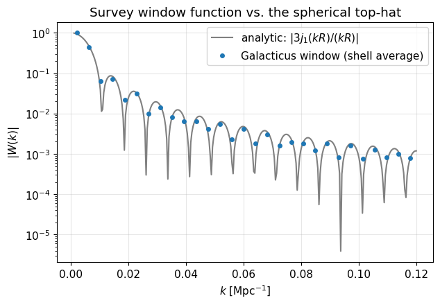
Here we use the all-sky geometry, whose selection volume for \(z \le 0.1\) is a solid sphere — so the exact answer is the classic spherical top-hat, \(W(k) = 3\,j_1(kR)/(kR)\), and we can validate the machinery three independent ways.

fullSky = galacticus.surveyGeometryFullSky(redshiftMinimum=0.0, redshiftMaximum=0.1,
                                           cosmologyFunctions_=cosmologyFunctions)
gridCount = 64
boxLength, window1, window2 = fullSky.windowFunctions(1.0e10, 1.0e10, gridCount)
radiusSurvey = fullSky.distanceMaximum(1.0e10)
print(f"box length      : {boxLength:8.2f} Mpc")
print(f"survey radius   : {radiusSurvey:8.2f} Mpc  (z=0.1)")
print(f"window grid     : {window1.shape}, dtype {window1.dtype}")
print(f"W(k=0)          : {window1[0,0,0]}")

# Validation 1: Galacticus's FFTW result vs numpy's FFT of the identically
# discretized selection function — must agree to machine precision.
x = (np.arange(1, gridCount+1)-0.5)*boxLength/gridCount - boxLength/2.0
X, Y, Z = np.meshgrid(x, x, x, indexing='ij')
selection = (np.sqrt(X**2+Y**2+Z**2) < radiusSurvey).astype(complex)
windowNumpy = np.fft.fftn(selection); windowNumpy /= windowNumpy[0,0,0]
error = np.max(np.abs(window1-windowNumpy))
print(f"max |W_Galacticus - W_numpy| = {error:.3e}")
assert error < 1.0e-10

box length      :  1255.99 Mpc
survey radius   :   418.66 Mpc  (z=0.1)
window grid     : (64, 64, 64), dtype complex128
W(k=0)          : (1+0j)
max |W_Galacticus - W_numpy| = 2.222e-16

# Validation 2: the radial profile of |W(k)| against the analytic
# spherical top-hat 3 j1(kR)/(kR).
kGrid = 2.0*np.pi*np.fft.fftfreq(gridCount, d=boxLength/gridCount)
KX, KY, KZ = np.meshgrid(kGrid, kGrid, kGrid, indexing='ij')
kMagnitude = np.sqrt(KX**2+KY**2+KZ**2)

def windowTopHat(k, R):
    x = np.maximum(k*R, 1.0e-10)
    return 3.0*(np.sin(x)-x*np.cos(x))/x**3

kBins  = np.linspace(0.0, 0.12, 30)
kMid   = 0.5*(kBins[1:]+kBins[:-1])
profile = np.array([np.mean(np.abs(window1)[(kMagnitude >= lo) & (kMagnitude < hi)])
                    for lo, hi in zip(kBins[:-1], kBins[1:])])
kSmooth = np.linspace(1.0e-3, 0.12, 300)
plt.plot(kSmooth, np.abs(windowTopHat(kSmooth, radiusSurvey)), color='gray',
         label='analytic: $|3 j_1(kR)/(kR)|$')
plt.plot(kMid, profile, 'o', ms=4, color='C0', label='Galacticus window (shell average)')
plt.yscale('log')
plt.xlabel('$k$ [Mpc$^{-1}$]'); plt.ylabel('$|W(k)|$')
plt.legend(); plt.title('Survey window function vs. the spherical top-hat')
plt.show()

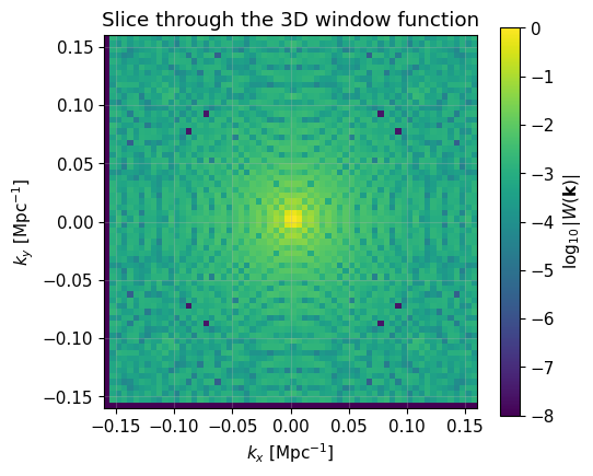
# Validation 3 (by eye): a slice through the 3D window — the ringing
# pattern of the top-hat transform.
plt.figure(figsize=(5.5, 4.6))
slicePlane = np.abs(np.fft.fftshift(window1)[:, :, gridCount//2])
kMax = np.abs(kGrid).max()
plt.imshow(np.log10(np.maximum(slicePlane, 1.0e-8)),
           extent=[-kMax, kMax, -kMax, kMax], origin='lower', cmap='viridis')
plt.colorbar(label='$\\log_{10} |W(\\mathbf{k})|$')
plt.xlabel('$k_x$ [Mpc$^{-1}$]'); plt.ylabel('$k_y$ [Mpc$^{-1}$]')
plt.title('Slice through the 3D window function')
plt.show()

A real survey’s window function

Mangle-based geometries build their window functions by Monte-Carlo sampling the polygon mask (polygons drawn in proportion to their solid angles, depths uniform in volume within the survey’s limits). This needs a random number generator — pass one to the survey’s constructor. The sampling takes a minute or so for the 200,000-polygon SDSS mask.

randomNumberGenerator = galacticus.randomNumberGeneratorGSL(
    seed_=8675309, ompThreadOffset=False, mpiRankOffset=False)
sdssSampled = galacticus.surveyGeometryBernardi2013SDSS(
    randomNumberGenerator_=randomNumberGenerator)
print(f"window functions available without RNG: {sdss.windowFunctionAvailable()}")
print(f"window functions available with    RNG: {sdssSampled.windowFunctionAvailable()}")

boxLengthSDSS, windowSDSS, _ = sdssSampled.windowFunctions(1.0e11, 1.0e11, gridCount)
print(f"box length: {boxLengthSDSS:.1f} Mpc,  W(0) = {windowSDSS[0,0,0]}")
assert windowSDSS[0,0,0] == 1.0+0j

kGridSDSS = 2.0*np.pi*np.fft.fftfreq(gridCount, d=boxLengthSDSS/gridCount)
kMaxSDSS  = np.abs(kGridSDSS).max()
fig, axes = plt.subplots(1, 2, figsize=(11, 4.4))
for ax, W, kM, label in ((axes[0], window1, np.abs(kGrid).max(), 'full sky ($z<0.1$)'),
                         (axes[1], windowSDSS, kMaxSDSS, 'SDSS (Bernardi+13)')):
    sliceW = np.abs(np.fft.fftshift(W)[:, :, W.shape[2]//2])
    im = ax.imshow(np.log10(np.maximum(sliceW, 1.0e-8)),
                   extent=[-kM, kM, -kM, kM], origin='lower', cmap='viridis')
    ax.set_xlabel('$k_x$ [Mpc$^{-1}$]'); ax.set_ylabel('$k_y$ [Mpc$^{-1}$]')
    ax.set_title(label)
    fig.colorbar(im, ax=ax, label=r'$\log_{10}|W|$')
fig.suptitle('Isotropic vs. real-survey window functions')
fig.tight_layout(); plt.show()

window functions available without RNG: False
window functions available with    RNG: True

<>:22: SyntaxWarning: "\l" is an invalid escape sequence. Such sequences will not work in the future. Did you mean "\\l"? A raw string is also an option.
<>:22: SyntaxWarning: "\l" is an invalid escape sequence. Such sequences will not work in the future. Did you mean "\\l"? A raw string is also an option.
/tmp/ipykernel_4017964/281119426.py:22: SyntaxWarning: "\l" is an invalid escape sequence. Such sequences will not work in the future. Did you mean "\\l"? A raw string is also an option.
  fig.colorbar(im, ax=ax, label='$\log_{10}|W|$')

box length: 3060.8 Mpc,  W(0) = (1+0j)

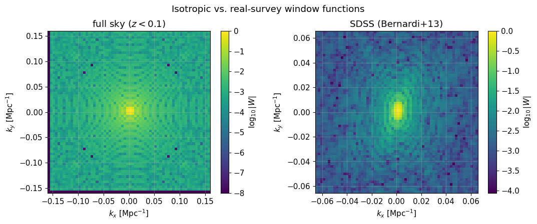
The full-sky window rings symmetrically; the SDSS window is visibly anisotropic — the imprint of the survey’s footprint on Fourier space.

Finale: convolving \(P(k)\) with the survey window

What a survey measures is not \(P(k)\) but its convolution with \(|W(\mathbf{k})|^2\):

\[P_\mathrm{obs}(\mathbf{k}) \;=\; \frac{\sum_{\mathbf{k}'} P(k')\,|W(\mathbf{k}-\mathbf{k}')|^2}{\sum_{\mathbf{k}'} |W(\mathbf{k}')|^2}.\]

We assemble the linear power spectrum from Tutorial 2, evaluate it on the full-sky window’s Fourier grid, and perform the convolution with FFTs. The window kernel \(|W|^2\) has width \(\Delta k \sim 2\pi/R\) where \(R\) is the survey extent — here a compact kernel, so the redistribution of power is at the few-per-cent level and largest where \(P(k)\) changes fastest (near the largest scales and the spectrum’s turnover). Shallower or narrower surveys have broader kernels and correspondingly stronger distortions — the machinery below applies unchanged.

# The linear power spectrum (Tutorial 2's object graph, condensed).
darkMatterParticle      = galacticus.darkMatterParticleCDM()
transferFunction        = galacticus.transferFunctionEisensteinHu1999(
    3.046, 0.0, darkMatterParticle, cosmologyParameters, cosmologyFunctions)
linearGrowth            = galacticus.linearGrowthCollisionlessMatter(cosmologyParameters, cosmologyFunctions)
powerSpectrumPrimordial = galacticus.powerSpectrumPrimordialPowerLaw(0.965, 0.0, 0.0, 1.0, False)
powerSpectrum           = galacticus.powerSpectrumPrimordialTransferredSimple(
    powerSpectrumPrimordial, transferFunction, linearGrowth)
ageToday = cosmologyFunctions.cosmicTime(1.0)

# Evaluate P(|k|) on the window's Fourier grid (binned by |k| for speed).
kFlat   = kMagnitude.ravel()
order   = np.argsort(kFlat)
pFlat   = np.zeros_like(kFlat)
kUnique, inverse = np.unique(np.round(kFlat, 12), return_inverse=True)
pUnique = np.array([powerSpectrum.power(k, ageToday) if k > 0.0 else 0.0
                    for k in kUnique])
pGrid   = pUnique[inverse].reshape(kMagnitude.shape)

# Circular convolution via the convolution theorem, normalized so that a
# constant spectrum is preserved.
windowSquared = np.abs(window1)**2
pConvolved = np.real(np.fft.ifftn(np.fft.fftn(pGrid)*np.fft.fftn(windowSquared)))
pConvolved /= np.sum(windowSquared)

# Shell-average both and compare.
kBins = np.linspace(kGrid[1]*0.5, 0.25, 40)
kMid  = 0.5*(kBins[1:]+kBins[:-1])
def shellAverage(field):
    return np.array([np.mean(field[(kMagnitude >= lo) & (kMagnitude < hi)])
                     for lo, hi in zip(kBins[:-1], kBins[1:])])
pTrue, pObs = shellAverage(pGrid), shellAverage(pConvolved)

fig, (axP, axR) = plt.subplots(2, 1, figsize=(7, 6.5), sharex=True,
                               gridspec_kw={'height_ratios': (3, 1)})
axP.loglog(kMid, pTrue, label='$P(k)$ (theory)')
axP.loglog(kMid, pObs , label='$P_{\\rm obs}(k)$ (window-convolved)')
axP.set_ylabel('$P$ [Mpc$^3$]'); axP.legend()
axP.set_title('Window convolution of the power spectrum')
axR.semilogx(kMid, pObs/pTrue); axR.axhline(1.0, color='gray', ls=':')
axR.set_xlabel('$k$ [Mpc$^{-1}$]'); axR.set_ylabel('obs / true')
fig.tight_layout(); plt.show()

# Quantitative signatures for this compact window: percent-level
# redistribution everywhere, approaching unity in the well-sampled
# intermediate range.
print(f"obs/true at k={kMid[0]:.4f}: {pObs[0]/pTrue[0]:.3f}")
print(f"obs/true at k={kMid[-1]:.3f}: {pObs[-1]/pTrue[-1]:.3f}")
assert np.all(np.abs(pObs/pTrue-1.0) < 0.20)
assert abs(pObs[-1]/pTrue[-1]-1.0) < 0.10

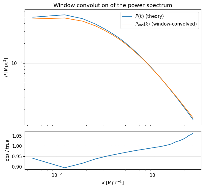
obs/true at k=0.0057: 0.941
obs/true at k=0.247: 1.064

Where next

Every mask operation here (pointIncluded above all) is exactly what Galacticus itself uses when constructing mock catalogues on lightcones, and the window-convolution above is the forward model for comparing Tutorial 2’s spectra — CDM or WDM — with survey measurements. For higher-fidelity survey windows, increase the grid size (and note that angularPower computes the mask’s spherical-harmonic decomposition from the polygon file on first use — an expensive, cached operation).